X <- read.table('data/Example1.dat', header = FALSE)
X <- as.matrix(X)
C <- scale(X, scale = FALSE)Dimension reduction 1 - Principal Components Analysis
Introduction
In this practical, we will perform singular value decomposition and perform principical component analysis. You will not have to load any packages in advance, as we will solely use base R. The data for todays practical can be downloaded here:
Take home exercises
SVD and Eigendecomposition
In this exercise, the data of Example 1 from the lecture slides are used. These data have been stored in the file Example1.dat.
1. Use the function read.table() to import the data into R. Use the function as.matrix() to convert the data frame to a matrix. The two features are not centered. To center the two features the function scale() with the argument scale = FALSE can be used. Give the centered data matrix a name, for instance, C.
2. Calculate the sample size N and the covariance matrix S by executing the following R code, where the function t() is used to calculate the transpose of C and %*% is used for matrix multiplication.
N <- dim(C)[1]
S <- t(C) %*% C/N
3. Use the function svd() to apply a singular value decomposition to the centered data matrix.
SVD <- svd(C)
SVD
$d
[1] 31.219745 5.032642
$u
[,1] [,2]
[1,] -0.26680000 0.28739123
[2,] -0.05470446 -0.33737580
[3,] -0.55896540 -0.13388431
[4,] -0.30683494 -0.23562992
[5,] -0.01466951 0.18564553
[6,] 0.19742603 -0.43912150
[7,] 0.48959143 -0.01784596
[8,] 0.02536542 0.70866669
[9,] 0.48959143 -0.01784596
$v
[,1] [,2]
[1,] 0.4289437 0.9033312
[2,] 0.9033312 -0.42894374. Inspect the three pieces of output, that is, U, D, and V. Are the three matrices the same as on the slides?
Note: A singular value decomposition is not unique. The singular values are unique, but the left and right singular vectors are only unique up to sign. This means that the singular vectors can be multiplied by -1 without changing the singular value decomposition.
5. Use a single matrix product to calculate the principal component scores.
U <- SVD$u
D <- diag(SVD$d)
V <- SVD$v
L <- C %*% V
L
[,1] [,2]
[1,] -8.3294282 1.44633709
[2,] -1.7078593 -1.69789153
[3,] -17.4507576 -0.67379177
[4,] -9.5793087 -1.18584098
[5,] -0.4579784 0.93428745
[6,] 6.1635905 -2.20994117
[7,] 15.2849198 -0.08981231
[8,] 0.7919021 3.56646553
[9,] 15.2849198 -0.08981231U %*% D [,1] [,2]
[1,] -8.3294282 1.44633709
[2,] -1.7078593 -1.69789153
[3,] -17.4507576 -0.67379177
[4,] -9.5793087 -1.18584098
[5,] -0.4579784 0.93428745
[6,] 6.1635905 -2.20994117
[7,] 15.2849198 -0.08981231
[8,] 0.7919021 3.56646553
[9,] 15.2849198 -0.089812316. Plot the scores on the second principal component (y-axis) against the scores on the first principal component (x-axis) and let the range of the x-axis run from -18 to 18 and the range of the y-axis from -16 to 16.
plot(L[,1],
     L[,2],
     xlim = c(-18, 18),
     ylim = c(-16, 16))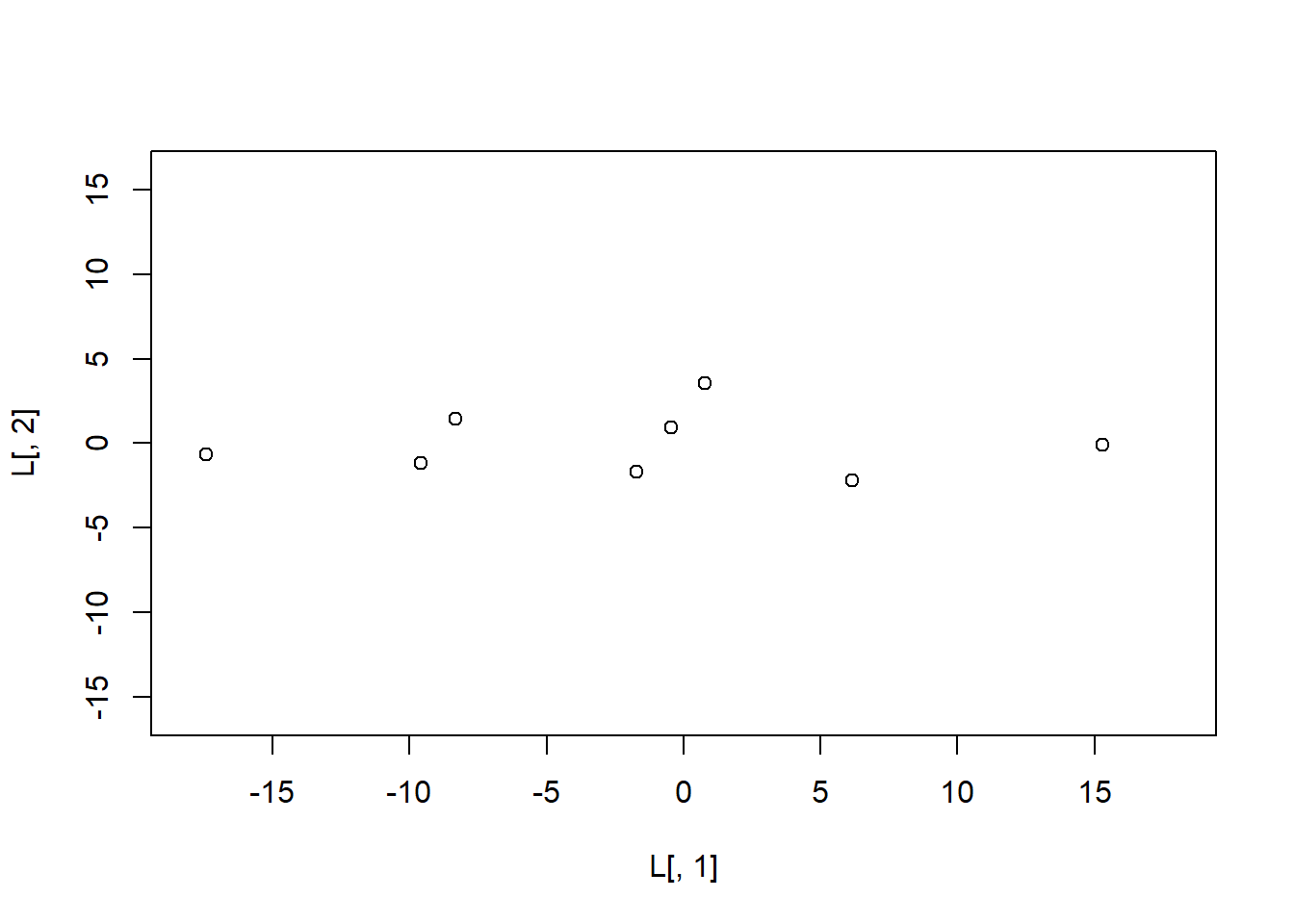
7. Use the function eigen() to apply an eigendecomposition to the sample covariance matrix.
Note that an alternative form of the eigendecomposition of the covariance matrix \(\mathbf{S}\) is given by

where \(\mathbf{v}_{j}\) is the \(j\)th eigenvector of \(\mathbf{S}\). From this alternative form it is clear that the (ortho-normal) eigenvectors are only defined up to sign because \(\mathbf{v}_{j}\mathbf{v}_{j}^{T}=-\mathbf{v}_{j}(-\mathbf{v}_{j}^{T})\). This may lead to differences in sign in the output.
eigen(S)eigen() decomposition
$values
[1] 108.296945 2.814165
$vectors
[,1] [,2]
[1,] 0.4289437 -0.9033312
[2,] 0.9033312 0.42894378. Check whether the eigenvalues are equal to the variances of the two principal components. Be aware that the R-base function var() takes \(N-1\) in the denominator, to get an unbiased estimate of the variance.
round((N - 1) * var(L)/N, 2) [,1] [,2]
[1,] 108.3 0.00
[2,] 0.0 2.819. Finally, calculate the percentage of total variance explained by each principal component.
round(diag((N - 1) * var(L)/N) / sum(diag((N - 1) * var(L)/N)) * 100, 2)[1] 97.47 2.53Principal component analysis
In this exercise, a PCA is used to determine the financial strength of insurance companies. Eight relevant features have been selected: (1) gross written premium, (2) net mathematical reserves, (3) gross claims paid, (4) net premium reserves, (5) net claim reserves, (6) net income, (7) share capital, and (8) gross written premium ceded in reinsurance.
To perform a principal component analysis, an eigendecomposition can be applied to the sample correlation matrix \(\mathbf{R}\) instead of the sample covariance matrix \(\mathbf{S}\). Note that the sample correlation matrix is the sample covariance matrix of the standardized features. These two ways of doing a PCA will yield different results. If the features have the same scales (the same units), then the covariance matrix should be used. If the features have different scales, then it’s better in general to use the correlation matrix because otherwise the features with high absolute variances will dominate the results.
The means and standard deviations of the features can be found in the following table.
| feature | mean | std.dev. |
|---|---|---|
| (1) GR_WRI_PRE | 143,232,114 | 228,320,220 |
| (2) NET_M_RES | 43,188,939 | 151,739,600 |
| (3) GR_CL_PAID | 65,569,646 | 125,986,400 |
| (4) ET_PRE_RES | 41,186,950 | 65,331,440 |
| (5) NET_CL_RES | 14,726,188 | 24,805,660 |
| (6) NET_INCOME | -1,711,048 | 22,982,140 |
| (7) SHARE_CAP | 33,006,176 | 38,670,760 |
| (8) R_WRI_PR_CED | 37,477,746 | 93,629,540 |
The sample correlation matrix is given below.
| (1) | (2) | (3) | (4) | (5) | (6) | (7) | (8) | |
|---|---|---|---|---|---|---|---|---|
| (1) | 1.00 | 0.32 | 0.95 | 0.94 | 0.84 | 0.22 | 0.47 | 0.82 |
| (2) | 0.32 | 1.00 | 0.06 | 0.21 | 0.01 | 0.30 | 0.10 | 0.01 |
| (3) | 0.95 | 0.06 | 1.00 | 0.94 | 0.89 | 0.14 | 0.44 | 0.81 |
| (4) | 0.94 | 0.21 | 0.94 | 1.00 | 0.88 | 0.19 | 0.50 | 0.68 |
| (5) | 0.84 | 0.01 | 0.89 | 0.88 | 1.00 | -0.23 | 0.55 | 0.63 |
| (6) | 0.22 | 0.30 | 0.14 | 0.19 | -0.23 | 1.00 | -0.15 | 0.21 |
| (7) | 0.47 | 0.10 | 0.44 | 0.50 | 0.55 | -0.15 | 1.00 | 0.14 |
| (8) | 0.82 | 0.01 | 0.81 | 0.68 | 0.63 | 0.21 | 0.14 | 1.00 |
R <- matrix(c(1.00,0.32,0.95,0.94,0.84,0.22,0.47,0.82,
              0.32,1.00,0.06,0.21,0.01,0.30,0.10,0.01,
              0.95,0.06,1.00,0.94,0.89,0.14,0.44,0.81,
              0.94,0.21,0.94,1.00,0.88,0.19,0.50,0.68,
              0.84,0.01,0.89,0.88,1.00,-0.23,0.55,0.63,
              0.22,0.30,0.14,0.19,-0.23,1.00,-0.15,0.21,
              0.47,0.10,0.44,0.50,0.55,-0.15,1.00,0.14,
              0.82,0.01,0.81,0.68,0.63,0.21,0.14,1.00),
            nrow = 8)
9. Use R to apply a PCA to the sample correlation matrix.
EVD <- eigen(R)
round(EVD$values, 2)
[1] 4.65 1.45 1.01 0.57 0.25 0.03 0.02 0.00round(EVD$vectors, 2) [,1] [,2] [,3] [,4] [,5] [,6] [,7] [,8]
[1,] 0.46 0.12 0.02 0.09 0.09 0.16 0.04 0.86
[2,] 0.09 0.52 0.65 0.49 0.10 0.03 -0.04 -0.20
[3,] 0.45 -0.02 -0.15 -0.02 -0.15 0.77 0.14 -0.36
[4,] 0.45 0.04 0.04 -0.05 -0.45 -0.50 0.57 -0.13
[5,] 0.42 -0.29 0.03 0.16 -0.30 -0.21 -0.75 -0.10
[6,] 0.06 0.73 -0.17 -0.57 -0.13 -0.05 -0.30 -0.03
[7,] 0.25 -0.29 0.58 -0.60 0.39 -0.02 0.01 -0.08
[8,] 0.37 0.11 -0.44 0.18 0.70 -0.27 0.01 -0.24An alternative criterion for extracting a smaller number of principal components \(m\) than the number of original variables \(p\) in applying a PCA to the sample correlation matrix, is the eigenvalue-greater-than-one rule. This rule says that \(m\) (the number of extracted principal components) should be equal to the number of eigenvalues greater than one. Since each of the standardized variables has a variance of one, the total variance is \(p\). If a principal component has an eigenvalue greater than one, than its variance is greater than the variance of each of the original standardized variables. Then, this principal component explains more of the total variance than each of the original standardized variables.
10. How many principal components should be extracted according to the eigenvalue-greater-than-one rule?
11. How much of the total variance does this number of extracted principal components explain?
round(cumsum(EVD$values) * 100/sum(EVD$values), 2)[1] 58.19 76.26 88.94 96.09 99.25 99.64 99.95 100.0012. Make a scree-plot. How many principal components should be extracted according to the scree-plot?
plot(EVD$values, type = 'l')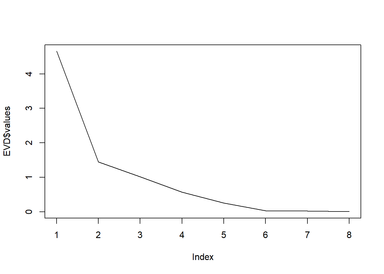
13. How much of the total variance does this number of extracted principal components explain?
14. Install the R-package keras, following the steps outlined here.
Note that the latest python version you can use is 3.11. It can be that you have to set the python interpreter in R Studio. This can be done at Tools > Global Options > Python.
Lab exercise
In this assignment, you will perform a PCA to a simple and easy to understand dataset. You will use the mtcars dataset, which is built into R. This dataset consists of data on 32 models of car, taken from an American motoring magazine (1974 Motor Trend magazine). For each car, you have 11 features, expressed in varying units (US units). They are as follows:
mpg: fuel consumption (miles per (US) gallon); more powerful and heavier cars tend to consume more fuel.cyl: number of cylinders; more powerful cars often have more cylinders.disp: displacement (cu.in.); the combined volume of the engine’s cylinders.hp: gross horsepower; this is a measure of the power generated by the car.drat: rear axle ratio; this describes how a turn of the drive shaft corresponds to a turn of the wheels. Higher values will decrease fuel efficiency.wt: weight (1000 lbs).qsec: 1/4 mile time, the cars speed and acceleration.vs: engine block; this denotes whether the vehicle’s engine is shaped like a ‘V’, or is a more common straight shape.am: transmission; this denotes whether the car’s transmission is automatic (0) or manual (1).gear: number of forward gears; sports cars tend to have more gears.carb: number of carburetors; associated with more powerful engines.
Note that the units used vary and occupy different scales.
First, the principal components will be computed. Because PCA works best with numerical data, you’ll exclude the two categorical variables (vs and am; columns 8 and 9). You are left with a matrix of 9 columns and 32 rows, which you pass to the prcomp() function, assigning your output to mtcars.pca. You will also set two arguments, center and scale, to be TRUE. This is done to apply a principal component analysis to the standardized features. So, execute
mtcars.pca <- prcomp(mtcars[, c(1:7, 10, 11)],
                     center = TRUE,
                     scale = TRUE)
15. Have a peek at the PCA object with summary().
summary(mtcars.pca)Importance of components:
PC1 PC2 PC3 PC4 PC5 PC6 PC7
Standard deviation 2.3782 1.4429 0.71008 0.51481 0.42797 0.35184 0.32413
Proportion of Variance 0.6284 0.2313 0.05602 0.02945 0.02035 0.01375 0.01167
Cumulative Proportion 0.6284 0.8598 0.91581 0.94525 0.96560 0.97936 0.99103
PC8 PC9
Standard deviation 0.2419 0.14896
Proportion of Variance 0.0065 0.00247
Cumulative Proportion 0.9975 1.00000You obtain 9 principal components, which you call PC1-9. Each of these explains a percentage of the total variance in the dataset.
16. What is the percentage of total variance explained by PC1?
17. What is the percentage of total variance explained by PC1, PC2, and PC3 together?
The PCA object mtcars.pca contains the following information:
- the center point or the vector of feature means (
$center) - the vector of feature standard deviations (
$scale) - the vector of standard deviations of the principal components (
$sdev) - the eigenvectors (
$rotation) - the principal component scores (
$x)
18. Determine the eigenvalues. How many principal components should be extracted according to the eigenvalue-greater-than-one rule?
round(mtcars.pca$sdev^2, 3)[1] 5.656 2.082 0.504 0.265 0.183 0.124 0.105 0.059 0.02219. What is the value of the total variance? Why?
20. How much of the total variance is explained by the number of extracted principal components according to the eigenvalue-greater-than-one rule?
Next, a couple of plots will be produced to visualize the PCA solution. You will make a biplot, which includes both the position of each observation (car model) in terms of PC1 and PC2 and also will show you how the initial features map onto this. A biplot is a type of plot that will allow you to visualize how the observations relate to one another in the PCA (which observations are similar and which are different) and will simultaneously reveal how each feature contributes to each principal component.
21. Use the function biplot() with the argument choices = c(1, 2) to ask for a biplot for the first two principal components.
biplot(mtcars.pca, choices = c(1, 2))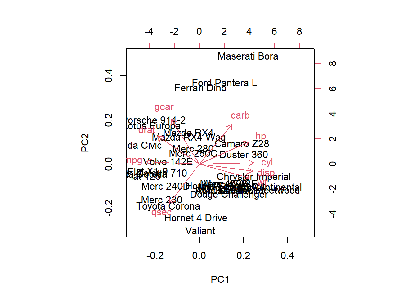
The axes of the biplot are seen as arrows originating from the center point. Here, you see that the variables hp, cyl, and disp all contribute to PC1, with higher values in those variables moving the observations to the right on this plot. This lets you see how the car models relate to the axes. You can also see which cars are similar to one another. For example, the Maserati Bora, Ferrari Dino and Ford Pantera L all cluster together at the top. This makes sense, as all of these are sports cars.
22. Make a biplot for the first and third principal components. Especially which brand of car has negative values on the first principal component and positive values on the third principal component?
biplot(mtcars.pca, choices = c(1, 3))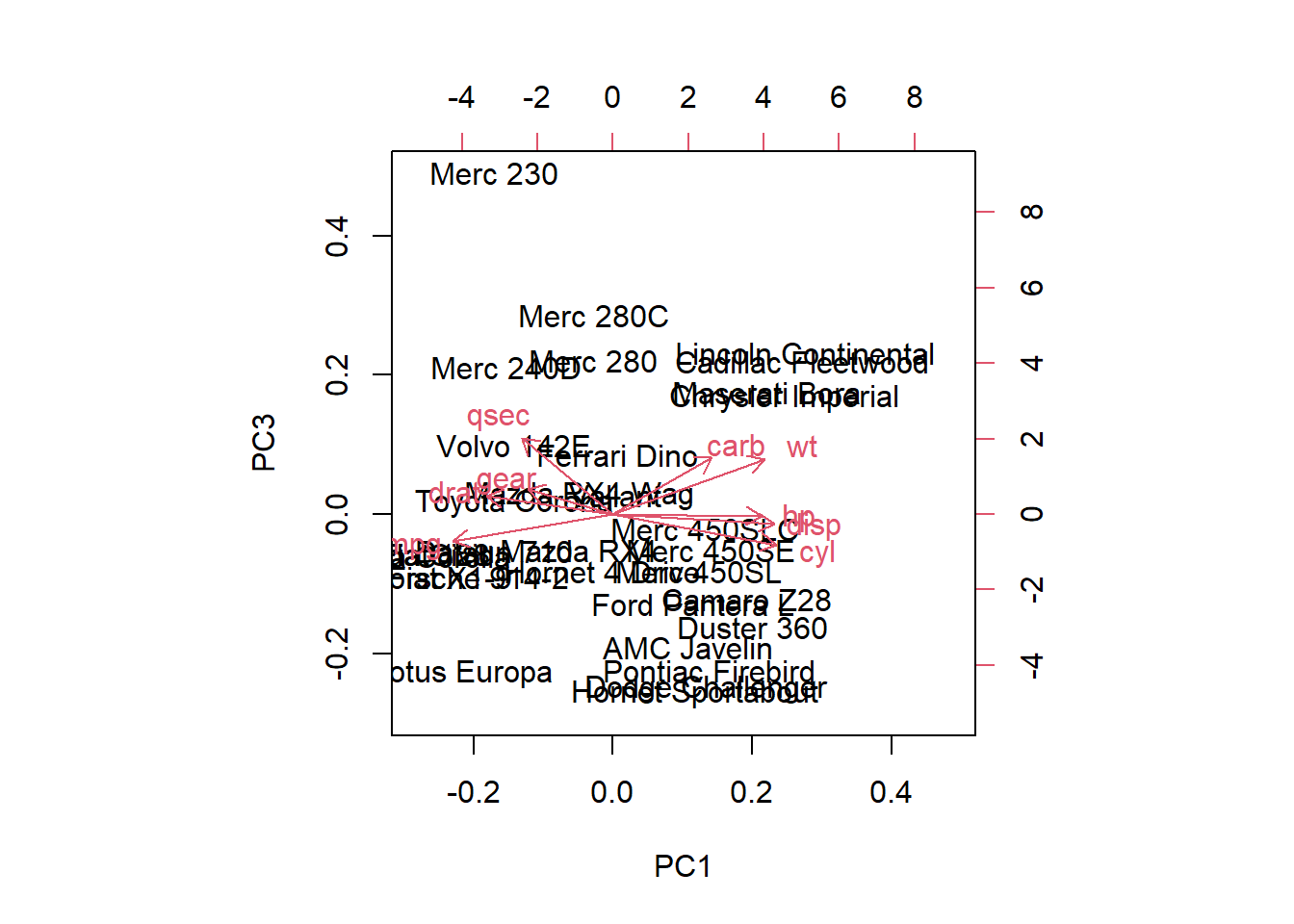
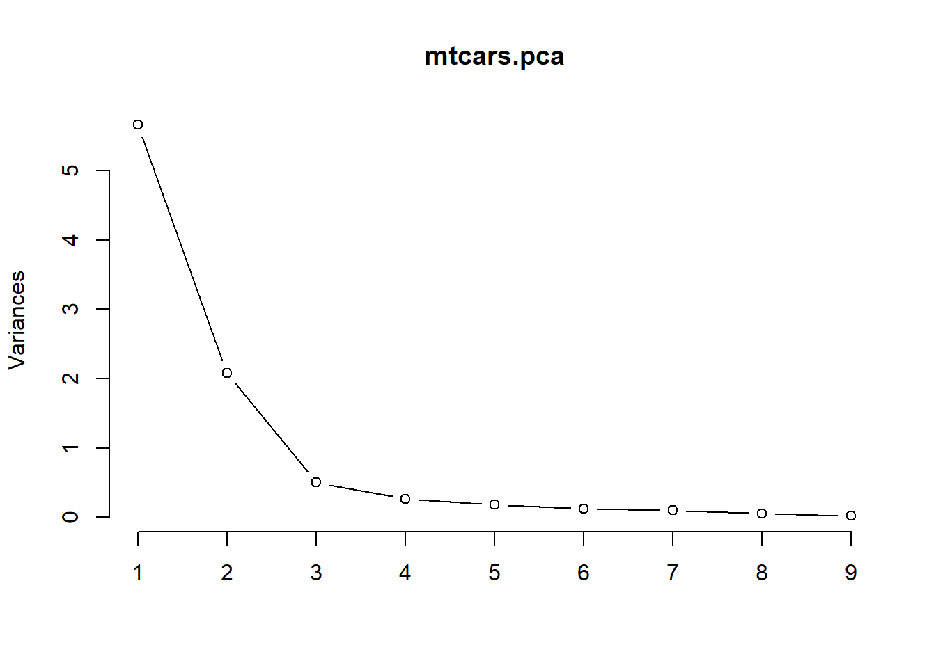
23. Use the function screeplot() with the argument type = 'lines' to produce a scree-plot. How many principal components should be extracted according to this plot? Why? Is this number in agreement with the number of principal components extracted according to the eigenvalue-greater-than-one rule?
screeplot(mtcars.pca, type = 'lines')