In this practical, we will learn word embeddings to represent text data, and we will also analyse a recurrent neural network.
We use the following packages:
Code
library(magrittr) # for pipeslibrary(tidyverse) # for tidy data and pipeslibrary(ggplot2) # for visualizationlibrary(wordcloud) # to create pretty word cloudslibrary(stringr) # for regular expressionslibrary(text2vec) # for word embeddinglibrary(tidytext) # for text mininglibrary(tensorflow)library(keras)
Take-home exercises
Word embedding
In the first part of the practical, we will apply word embedding approaches. A key idea in working with text data concerns representing words as numeric quantities. There are a number of ways to go about this as we reviewed in the lecture. Word embedding techniques such as word2vec and GloVe use neural networks approaches to construct word vectors. With these vector representations of words we can see how similar they are to each other, and also perform other tasks such as sentiment classification.
Let’s start the word embedding part with installing the harrypotter package using devtools. The harrypotter package supplies the first seven novels in the Harry Potter series. You can install and load this package with the following code:
Code
#devtools::install_github("bradleyboehmke/harrypotter")library(harrypotter) # Not to be confused with the CRAN palettes package
1. Use the code below to load the first seven novels in the Harry Potter series.
Code
hp_books <-c("philosophers_stone", "chamber_of_secrets","prisoner_of_azkaban", "goblet_of_fire","order_of_the_phoenix", "half_blood_prince","deathly_hallows")hp_words <-list( philosophers_stone, chamber_of_secrets, prisoner_of_azkaban, goblet_of_fire, order_of_the_phoenix, half_blood_prince, deathly_hallows) %>%# name each list elementset_names(hp_books) %>%# convert each book to a data frame and merge into a single data framemap_df(as_tibble, .id ="book") %>%# convert book to a factormutate(book =factor(book, levels = hp_books)) %>%# remove empty chaptersfilter(!is.na(value)) %>%# create a chapter id columngroup_by(book) %>%mutate(chapter =row_number(book))head(hp_words)## # A tibble: 6 × 3## # Groups: book [1]## book value chapter## <fct> <chr> <int>## 1 philosophers_stone "THE BOY WHO LIVED Mr. and Mrs. Dursley, of num… 1## 2 philosophers_stone "THE VANISHING GLASS Nearly ten years had passe… 2## 3 philosophers_stone "THE LETTERS FROM NO ONE The escape of the Braz… 3## 4 philosophers_stone "THE KEEPER OF THE KEYS BOOM. They knocked agai… 4## 5 philosophers_stone "DIAGON ALLEY Harry woke early the next morning… 5## 6 philosophers_stone "THE JOURNEY FROM PLATFORM NINE AND THREE-QUARTERS… 6
2. Convert the hp_words object into a dataframe and use the unnest_tokens() function from the tidytext package to tokenize the dataframe.
Code
# tokenize the data framehp_words <-as.data.frame(hp_words) %>%unnest_tokens(word, value)head(hp_words)## book chapter word## 1 philosophers_stone 1 the## 2 philosophers_stone 1 boy## 3 philosophers_stone 1 who## 4 philosophers_stone 1 lived## 5 philosophers_stone 1 mr## 6 philosophers_stone 1 and
3. Remove the stop words from the tokenized data frame.
4. Creates a vocabulary of unique terms using the create_vocabulary() function from the text2vec package and remove the words that they appear less than 5 times.
5. The next step is to create a token co-occurrence matrix (TCM). The definition of whether two words occur together is arbitrary. First create a vocab_vectorizer, then use a window of 5 for context words to create the TCM.
Code
# maps words to indicesvectorizer <-vocab_vectorizer(hp_vocab)# use window of 10 for context wordshp_tcm <-create_tcm(it, vectorizer, skip_grams_window =5)dim(hp_tcm)## [1] 8630 8630
6. Use the GlobalVectors as given in the code below to fit the word vectors on our data set. Choose the embedding size (rank variable) equal to 50, and the maximum number of co-occurrences equal to 10. Train word vectors in 20 iterations. You can check the full input arguments of the fit_transform function from here.
Code
glove <- GlobalVectors$new(rank =50, x_max =10)hp_wv_main <- glove$fit_transform(hp_tcm, n_iter =20, convergence_tol =0.001)## INFO [15:00:04.348] epoch 1, loss 0.1201## INFO [15:00:04.499] epoch 2, loss 0.0783## INFO [15:00:04.641] epoch 3, loss 0.0679## INFO [15:00:04.782] epoch 4, loss 0.0618## INFO [15:00:04.921] epoch 5, loss 0.0575## INFO [15:00:05.069] epoch 6, loss 0.0543## INFO [15:00:05.226] epoch 7, loss 0.0518## INFO [15:00:05.374] epoch 8, loss 0.0498## INFO [15:00:05.517] epoch 9, loss 0.0482## INFO [15:00:05.661] epoch 10, loss 0.0468## INFO [15:00:05.806] epoch 11, loss 0.0456## INFO [15:00:05.952] epoch 12, loss 0.0446## INFO [15:00:06.098] epoch 13, loss 0.0437## INFO [15:00:06.242] epoch 14, loss 0.0429## INFO [15:00:06.386] epoch 15, loss 0.0422## INFO [15:00:06.531] epoch 16, loss 0.0416## INFO [15:00:06.671] epoch 17, loss 0.0410## INFO [15:00:06.814] epoch 18, loss 0.0405## INFO [15:00:06.960] epoch 19, loss 0.0400## INFO [15:00:07.105] epoch 20, loss 0.0396
7. The GloVe model learns two sets of word vectors: main and context. Essentially they are the same since the model is symmetric. From the experience learning two sets of word vectors leads to higher quality embeddings (read more here). Best practice is to combine both the main word vectors and the context word vectors into one matrix. Extract the word vectors and save the summation of them for further questions.
Code
dim(hp_wv_main)## [1] 8630 50hp_wv_context <- glove$componentsdim(hp_wv_context)## [1] 50 8630# Either word-vectors matrices could work, but the developers of the technique suggest the sum/mean may work betterhp_word_vectors <- hp_wv_main +t(hp_wv_context)dim(hp_word_vectors)## [1] 8630 50
8. Find the most similar words to words “harry”, “death”, and “love”. Use the sim2 function with the cosine similary measure.
Code
harry <- hp_word_vectors["harry", , drop = F]cos_sim_rom <-sim2(x = hp_word_vectors, y = harry, method ="cosine", norm ="l2")head(sort(cos_sim_rom[,1], decreasing = T), 10)## harry ron hermione moment time looked quickly ## 1.0000000 0.8667391 0.8623137 0.8209236 0.8201845 0.7690142 0.7681430 ## left happened dumbledore ## 0.7657225 0.7393362 0.7185179death <- hp_word_vectors["death", , drop = F]cos_sim_rom <-sim2(x = hp_word_vectors, y = death, method ="cosine", norm ="l2")head(sort(cos_sim_rom[,1], decreasing = T), 10)## death eaters eater voldemort escaped voldemort's ## 1.0000000 0.9473222 0.8886765 0.6598957 0.6258171 0.5619242 ## fight yelled lord people ## 0.5611892 0.5384620 0.5292734 0.5147428love <- hp_word_vectors["love", , drop = F]cos_sim_rom <-sim2(x = hp_word_vectors, y = love, method ="cosine", norm ="l2")head(sort(cos_sim_rom[,1], decreasing = T), 10)## love ingredients potion horcruxes hunt bothered ## 1.0000000 0.5519101 0.5482892 0.5233350 0.5223741 0.5120451 ## potions realise lessons easy ## 0.5020931 0.4923215 0.4852735 0.4824427
9. Now you can play with word vectors! For example, add the word vector of “harry” with the word vector of “love” and subtract them from the word vector of “death”. What are the top terms in your result?
Code
test <- hp_word_vectors["harry", , drop = F] - hp_word_vectors["death", , drop = F] + hp_word_vectors["love", , drop = F]cos_sim_test <-sim2(x = hp_word_vectors, y = test, method ="cosine", norm ="l2")head(sort(cos_sim_test[,1], decreasing = T), 10)## harry hermione ron thinking muttered time er weasley ## 0.6582883 0.6350198 0.6141246 0.5998959 0.5833623 0.5522759 0.5499507 0.5453136 ## love quickly ## 0.5417902 0.5401518
Lab exercises
Sentiment classification with RNN
For sentiment classification with pre-trained word vectors, we want to use GloVe pretrained word vectors. These word vectors were trained on Wikipedia 2014 and Gigaword 5 containing 6B tokens, 400K vocab, uncased, 50d, 100d, 200d, & 300d vectors. Download the glove.6B.300d.txt file manually from the website or use the code below for this purpose.
Code
# Download Glove vectors if necessary# if (!file.exists('glove.6B.zip')) {# download.file('https://nlp.stanford.edu/data/glove.6B.zip',destfile = 'glove.6B.zip')# unzip('data/glove.6B.zip')# }
10. Use the code below to load the pre-trained word vectors from the file ‘glove.6B.300d.txt’ (if you have memory issues load the file ‘glove.6B.50d.txt’ instead).
11. IMDB movie reviews is a labeled data set available with the text2vec package. This data set consists of 5000 IMDB movie reviews, specially selected for sentiment analysis. The sentiment of the reviews is binary, meaning an IMDB rating < 5 results in a sentiment score of 0, and a rating >=7 has a sentiment score of 1. No individual movie has more than 30 reviews. Load this data set and convert it to a dataframe.
Code
# load an example dataset from text2vecdata("movie_review")as_tibble(movie_review)## # A tibble: 5,000 × 3## id sentiment review ## <chr> <int> <chr> ## 1 5814_8 1 "With all this stuff going down at the moment with MJ i've…## 2 2381_9 1 "\\\"The Classic War of the Worlds\\\" by Timothy Hines is…## 3 7759_3 0 "The film starts with a manager (Nicholas Bell) giving wel…## 4 3630_4 0 "It must be assumed that those who praised this film (\\\"…## 5 9495_8 1 "Superbly trashy and wondrously unpretentious 80's exploit…## 6 8196_8 1 "I dont know why people think this is such a bad movie. It…## 7 7166_2 0 "This movie could have been very good, but comes up way sh…## 8 10633_1 0 "I watched this video at a friend's house. I'm glad I did …## 9 319_1 0 "A friend of mine bought this film for 1, and even then it…## 10 8713_10 1 "<br /><br />This movie is full of references. Like \\\"Ma…## # ℹ 4,990 more rows
12. To create a learning model using Keras, let’s first define the hyperparameters. Define the parameters of your Keras model with a maximum of 10000 words, maxlen of 60 and word embedding size of 300 (if you had memory problems change the embedding dimension to a smaller value, e.g., 50).
Code
max_words <-1e4maxlen <-60dim_size <-300
13. Use the text_tokenizer function from Keras and tokenize the imdb review data using a maximum of 10000 words.
Code
# tokenize the input data and then fit the created objectword_seqs <-text_tokenizer(num_words = max_words) %>%fit_text_tokenizer(movie_review$review)
14. Transform each text into a sequence of integers (word indices) and use the pad_sequences function to pad the sequences.
Code
# apply tokenizer to the text and get indices instead of words# later pad the sequencex_train <-texts_to_sequences(word_seqs, movie_review$review) %>%pad_sequences(maxlen = maxlen)
15. Convert the sequence into a dataframe.
Code
# unlist word indicesword_indices <-unlist(word_seqs$word_index)# then place them into data.framedic <-data.frame(word =names(word_indices), key = word_indices, stringsAsFactors =FALSE) %>%arrange(key) %>%filter(row_number() <= max_words)
16. Use the code below to join the dataframe of sequences (word indices) from the IMDB reviews with GloVe pre-trained word vectors.
Code
# join the words with GloVe vectors and# if a word does not exist in GloVe, then fill NA's with 0word_embeds <- dic %>%left_join(vectors) %>%select(starts_with("dim")) %>%replace(., is.na(.), 0) %>%as.matrix()## Joining with `by = join_by(word)`
17. Extract the outcome variable from the sentiment column in the original dataframe and name it y_train.
Code
# the outcome variabley_train <-as.matrix(movie_review$sentiment)
18. Use the Keras functional API and create a recurrent neural network model as below. Can you describe this model?
Code
# Use Keras Functional APIinput <-layer_input(shape =list(maxlen), name ="input")model <- input %>%layer_embedding(input_dim = max_words, output_dim = dim_size, input_length = maxlen,# put weights into list and do not allow trainingweights =list(word_embeds), trainable =FALSE) %>%layer_spatial_dropout_1d(rate =0.2) %>%bidirectional(layer_gru(units =80, return_sequences =TRUE) )max_pool <- model %>%layer_global_max_pooling_1d()ave_pool <- model %>%layer_global_average_pooling_1d()output <-layer_concatenate(list(ave_pool, max_pool)) %>%layer_dense(units =1, activation ="sigmoid")model <-keras_model(input, output)# model summarymodel## Model: "model"## ________________________________________________________________________________## Layer (type) Output Shape Para Connected to Trainable ## m # ## ================================================================================## input (InputLayer [(None, 60)] 0 [] Y ## ) ## embedding (Embedd (None, 60, 300) 3000 ['input[0][0]'] N ## ing) 000 ## spatial_dropout1d (None, 60, 300) 0 ['embedding[0][0]' Y ## (SpatialDropout1 ] ## D) ## bidirectional (Bi (None, 60, 160) 1833 ['spatial_dropout1 Y ## directional) 60 d[0][0]'] ## global_average_po (None, 160) 0 ['bidirectional[0] Y ## oling1d (GlobalAv [0]'] ## eragePooling1D) ## global_max_poolin (None, 160) 0 ['bidirectional[0] Y ## g1d (GlobalMaxPoo [0]'] ## ling1D) ## concatenate (Conc (None, 320) 0 ['global_average_p Y ## atenate) ooling1d[0][0]', ## 'global_max_pooli ## ng1d[0][0]'] ## dense (Dense) (None, 1) 321 ['concatenate[0][0 Y ## ]'] ## ================================================================================## Total params: 3183681 (12.14 MB)## Trainable params: 183681 (717.50 KB)## Non-trainable params: 3000000 (11.44 MB)## ________________________________________________________________________________
19. Compile the model with an ‘adam’ optimizer, and the binary_crossentropy loss. You can choose accuracy or AUC for the metrics.
Code
# instead of accuracy we can use "AUC" metrics from "tensorflow.keras"model %>%compile(optimizer ="adam", # optimizer = optimizer_rmsprop(),loss ="binary_crossentropy",metrics = tensorflow::tf$keras$metrics$AUC() # metrics = c('accuracy'))
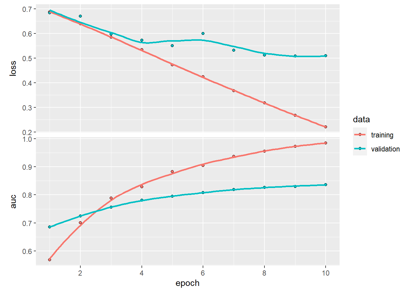
20. Fit the model with 10 epochs (iterations), batch_size = 32, and validation_split = 0.2. Check the training performance versus the validation performance.